Welcome back, stats adventurer! 👋 If you are here, it means you have already gone through our tutorial on: Linear models, Linear mixed effect models. Well done!! You are nearly there, my young stats padawan.
You might think that once you’ve fit the model, you’re basically done: check the summary, look for stars, write the results. But there’s a catch: If we just look at summary(), we will know whether effects exist (yes or no), but we still won’t be able to describe them in detail.
For example, if we find a significant interaction, we still don’t know the pattern that produced it. This is exactly what happened in our previous tutorial on mixed-effect models. Our hypothesis was simple: looking time differs across conditions (Simple vs Complex) but this difference might change over trials.
Need a refresher?
In our example paradigm, we designed a task where infants were presented with either a Simple or a Complex shape, and each shape was presented multiple times (that is, in multiple trials). We wanted to see if infants would look longer at the Complex shape, which would indicate increase interest for it over the Simple one. However, we were also mindful that this relationship might change (either get stronger or weaker) across trials. You can find an in-depth description of the experimental paradigm in our intro tutorial.
Even if we find a significant interaction between Condition (Simple vs Complex) and Trial Number, we still don’t know what exactly is happening: is looking time significantly decreasing over trials in the Simple condition? Or is it increasing in the Complex condition? Or is looking time changing in both condition, but at different rates? Let’s formulate our questions a bit more clearly:
What is the difference in Looking Time between Simple and Complex condition? ❓
At which trials are the conditions reliably different? ❓
Are the slopes across trials significantly different between conditions? ❓
Is the change in looking time over trials significant for both conditions? ❓
Luckily for us, there is a solution to this: we can further describe what the main and interaction effects look like, and we can even confidently say - backed by statistics - which differences are significant.
That’s the goal of this next tutorial. We will show how to visualise and test the specific effects you care about using model-based estimated means, contrasts, and slopes, so you can make clear statements about where and how conditions differ!
Setting things up
First let’s set things up to re-run our model. We import relevant libraries, read the data, set categorical variables as factors, standardize the continuous variables, and finally run our model.
Wait a sec, we just got an email…
I guess we have to listen to Reviewer #2 this time. Let’s include an additional interaction with SES (Socio-Economic Status) in our model. This variable is a factor with 3 levels: high, medium, and low. The serendipitous thing is that this complex model will be useful to fully understand how model’s predictions and estimates work, even when things get more complicated.
Inbox
Here’s our new model:
library(lme4)library(lmerTest)library(easystats)library(tidyverse)df=read.csv("resources/Stats/Dataset.csv")df$Id=factor(df$Id)# make sure subject_id is a factordf$SES=factor(df$SES)# make sure subject_id is a factordf$Event=factor(df$Event)# make sure subject_id is a factordf$StandardTrialN=standardize(df$TrialN)# create standardize trial columnmod=lmer(LookingTime~StandardTrialN*Event*SES+(1+StandardTrialN|Id), data=df)parameters(mod)
We now have three variables interacting with each other (a three-way interaction). Be careful when adding too many interactions! As explained in this blog post, the sample size you need increases very quickly when you do that.
Luckily for us, we are working on simulated data and, at least for these tutorials, we can get as much data as we want (* evil laugh *)
Model predictions
Remember how easy it was to draw lines in the first tutorial on linear models!? Back then, a model with one or two predictors was something you could sketch by hand. But now, with multiple interactions and random effects, trying to “draw the model” with would quickly become a mess.
Luckily, instead of pen and paper, we can ask the model to make predictions for us. That way, the model draws the lines while we sit back and relax. 😌
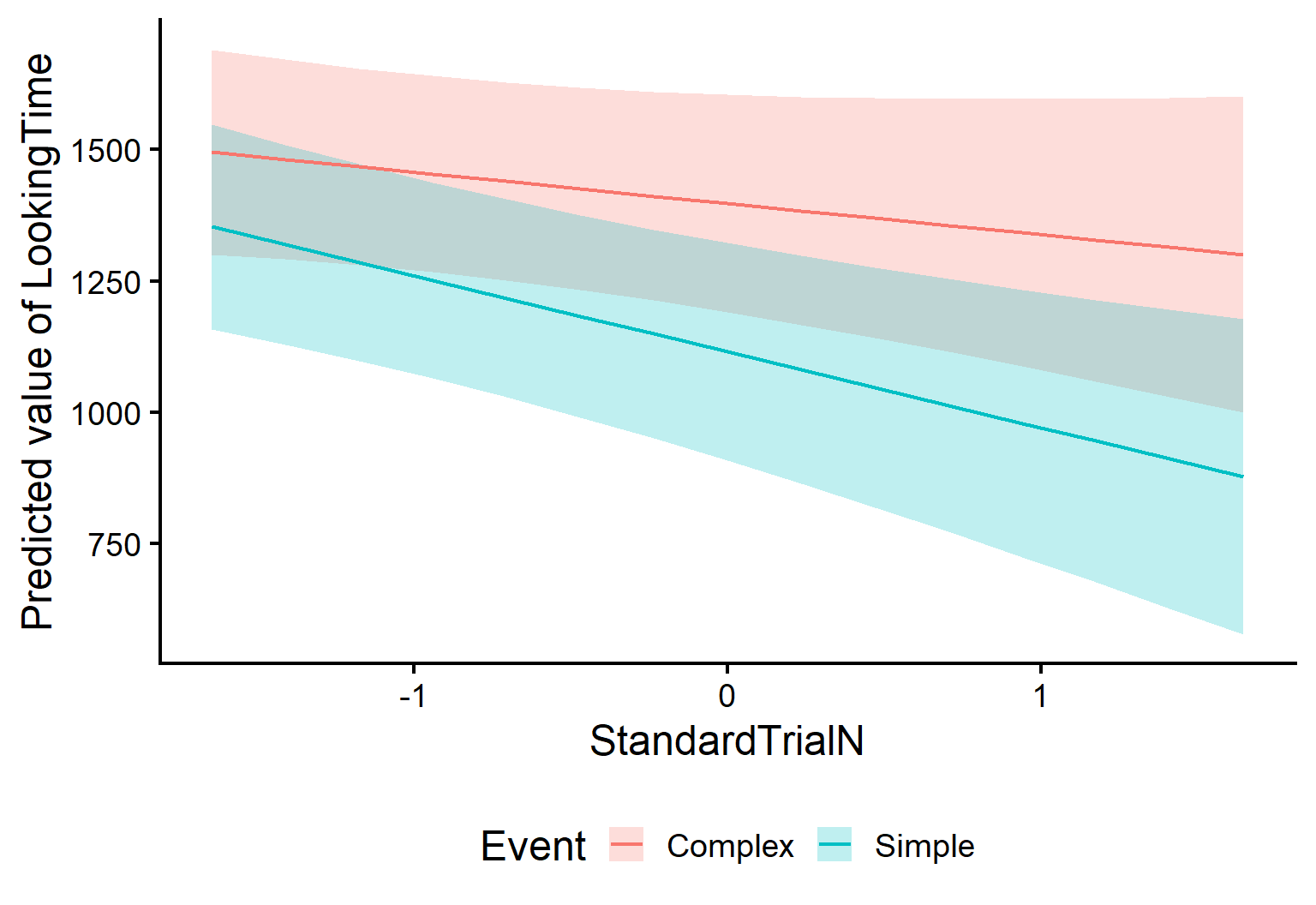
Predictions are simply the values of LookingTime that the model expects under specific conditions (e.g., Simple vs Complex Condition, early vs late trials).
We’ll use estimate_expectation() (from modelbased) to get predicted values directly from the fitted model. If we want to ask for predictions across Conditions and Trials, we can specify the following in the argument by (length tells how many values of the continuous predictor(s) to use):
As you can see, we get a Predicted value of looking time for each trial and event value! All without doing any mental arithmetics. Now we can plot these predictions to visualise the model-implied lines:
Have you spotted anything odd in the previous output!??
Well, look at the table with the model’s predictions. Just below it, we see the following:
Predictors controlled: SES (high)
We gotta be careful! These predictions do not apply for all SES levels! When we ask for predictions “by Event and Trial”, the model still needs to decide what to do with everything else in the model (like SES, and the random effects). By default, predictions are computed at specific values (e.g., reference levels for factors), so they may not represent the “mean” effect you want to report.
Tip
In this tutorial, we only introduce Prediction briefly because we care about means effects and contrasts more. However, you can always learn more on the modelbased website !!
Predictions help us describe patterns (“the lines diverge”, “one looks steeper”), but they don’t directly answer the questions about our initial hypothesis we care about:
What is the average difference between Simple and Complex (overall, not at one SES level)? ❓
At which trials are the conditions reliably different? ❓
Are the slopes across trials significantly different between conditions? ❓
Is the change in looking time over trials significant for both conditions? ❓
For that, we need model-based estimates that are designed for inference: estimated means, contrasts, and slopes - with uncertainty (CIs) and tests.
In the next section, we’ll start with estimated marginal means (averaged over the other predictors), and then use contrasts to formally test the specific differences we care about.
Estimate means
As its name suggests, estimate_means() allows you to extract estimated means from your model. But what does this actually mean? (Yes, lots of “means” in this explanation!)
This function:
Generates predictions for all the reference levels of a model’s predictors
Averages these predictions to keep only the predictors we are interested in
Think of it as a streamlined way to answer the question: “What is the average looking time for each level of my factor, according to my model?” Let’s see it in action!!
Estimated Marginal Means

Event   |    Mean |    SE |             95% CI | t(364)
-------------------------------------------------------
Complex | 1420.76 | 58.22 | [1306.27, 1535.25] |  24.40
Simple  | 1144.30 | 58.22 | [1029.81, 1258.79] |  19.65

Variable predicted: LookingTime
Predictors modulated: Event
Predictors averaged: StandardTrialN (0.005), SES, Id
Notice the information message! Previously, with estimate_expectation(), we were setting SES to its reference level (“high”). Now instead, the function extracts predictions for all levels of SES and then averages across them!, giving you a comprehensive view of how Event influences looking behavior.
THIS IS WHAT WE WANTED!!! 🎉🎉🎉
Note
estimate_expectation() and estimate_means() handle the random effect structure differently. By default, estimate_means() gives us an average effect of the predictor for an average subject - exactly what we need when trying to understand overall patterns in our data. Learn more with this vignette
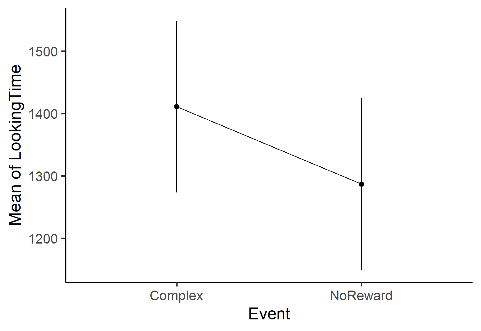
Easy plotting
The estimate_means() function also comes with its own built-in plotting capability, automatically generating a clean ggplot visualization of your estimated means.
We’ve successfully extracted and plotted the estimated means for our predictors - awesome job! 🎉
But there’s something important missing. While we now know the estimated looking times for each level, we don’t yet have formal statistical comparisons between these levels. For example, is the difference between mean values in Complex condition and Simple condition statistically significant?
Marginal Contrasts Analysis

Level1 | Level2  | Difference |   SE |             95% CI | t(364) |      p
---------------------------------------------------------------------------
Simple | Complex |    -276.46 | 6.07 | [-288.39, -264.53] | -45.58 | < .001

Variable predicted: LookingTime
Predictors contrasted: Event
Predictors averaged: StandardTrialN (0.005), SES, Id
p-values are uncorrected.
What we’re doing here is simple but powerful:
We pass our model to the function
We specify which predictor we want to compare (Event)
The function returns the difference between the means of the predictors with statistical tests
The results show us that the difference between Complex and Simple is positive (meaning looking time is higher for Complex) and the p-value indicates this difference is statistically significant! All of this with just one line of code - how convenient!
In this example, Event has only 2 levels (Complex and Simple), so we already knew these levels differed significantly from examining our model summary. However, estimate_contrast() becomes particularly powerful when dealing with predictors that have multiple levels. With a predictor like SES (3 levels) - estimate_contrast() automatically calculates all possible pairwise comparisons between these levels.
Note
Remember that if you have multiple levels in predictors you will need to adjust the p-value for multiple comparisons. You can do that by passing the argument p_adjust = 'hochberg' to the function. There are different adjustment methods and you can check them here.
Marginal Contrasts Analysis

Level1 | Level2 | Difference |     SE |            95% CI | t(364) |     p
--------------------------------------------------------------------------
low    | high   |      67.18 | 139.14 | [-206.45, 340.81] |   0.48 | 0.934
medium | high   |      12.41 | 148.75 | [-280.10, 304.93] |   0.08 | 0.934
medium | low    |     -54.76 | 139.14 | [-328.39, 218.86] |  -0.39 | 0.934

Variable predicted: LookingTime
Predictors contrasted: SES
Predictors averaged: StandardTrialN (0.005), Event, Id
p-value adjustment method: Hochberg (1988)
See?? We have all the comparison between the available level of SES. Ough, nothing is significant here - Reviewer #2 really made us work for nothing. Well, hopefully it’ll make them happy to know we listended to them. And on the upside, if we will even need to test differences between 3 or more groups, we’ll know exactly how to do that!
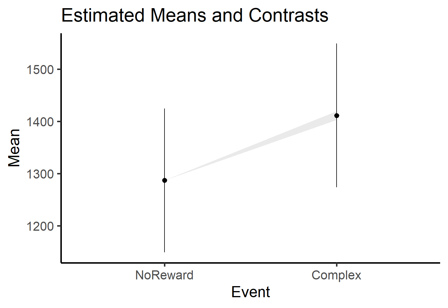
Almost-as-Easy plotting
estimate_contrast() has a plotting function as well! However, it’s slightly more complex as the plot function requires both our estimated contrasts and means. If we pass both, the plot will show which level is different from the other using lighthouse plots - visualizations that highlight significant differences between groups.
We hope you are getting a hang of how estimate_contrast() works. It helped us testing the first part of our hypothesis (and even check the effect of SES), but if we look back at our questions, two more aspects are still unclear:
What is the average difference between Simple and Complex (overall, not at one SES level)? ✅About 300ms, and the difference is significant!
At which trials are the conditions reliably different? ❓
Are the slopes across trials significantly different between conditions? ❓
Is the change in looking time over trials significant for both conditions? ❓
Luckily for us, estimate_contrast() really shines the most when examining interactions between categorical and continuous predictors - just what we want. More specifically, we care about whether the effect of Condition (Event), changes across Trials. So we can keep contrast = Event. But now we also want to compute that difference across trials! For that, we can use by =. Here’s how it works:
contrast = tells the function what difference you want to compute (e.g., Complex vs Simple).
by = tells it where to compute that difference (at different trial values).
ContrastbyTrial=estimate_contrasts(mod, contrast ='Event', by ='StandardTrialN', p_adjust ='hochberg')ContrastbyTrial
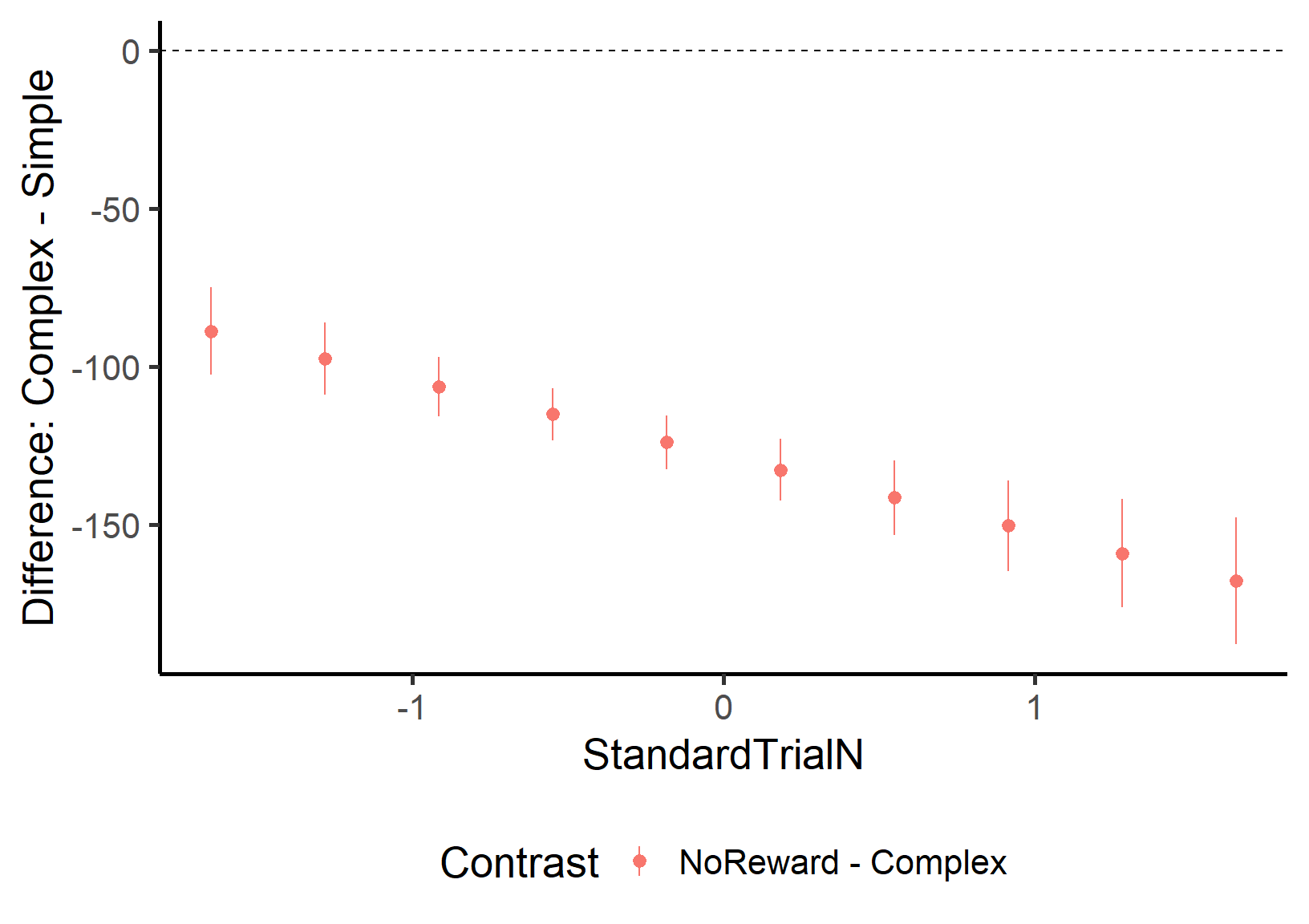
This gives us the contrast between the levels of Event for a set of values of StandardTrialN. So we can check whether the difference between Complex and Simple actually changes over the course of trials!! We’ll plot it to make it simpler to understand:
This plot shows that the two levels are always significantly different from each other (the confidence intervals never touch the dashed zero line) and that the difference is always positive - looking time for Complex is consistently higher than for Simple across all trial numbers. SUUPER COOL, EH!!?
Important
You can put multiple predictors in contrast = (it will compute lots of pairwise differences across combinations), but be careful: the number of tests can explode fast… and you’ll want p-value adjustment.
Comparing slopes
Wow, it took a while to get here, but now we’re quickly answering all of our questions! We’re already half-way through:
What is the average difference between Simple and Complex (overall, not at one SES level)? ✅About 300ms, and the difference is significant!
At which trials are the conditions reliably different? ✅All of them!
Are the slopes across trials significantly different between conditions? ❓
Is the change in looking time over trials significant for both conditions? ❓
To answer the next question, we can again use the estimate_contrast() function. However, we need to make a fundamental change. Before, we cared about how the effect of Condition changed across Trials. Now, we care about how the effect of Trial changes across conditions!
Is that super confusing? It still is for us, sometimes. But remembering our question helps: Does the effect of time (Trial) change across Conditions? For that, our main interest is Trial Number, and we want to see how the experimental condition modulates it. So StandardTrialN moves to the contrast argument and Event goes to the by argument:
Marginal Contrasts Analysis

Level1 | Level2  | Difference |   SE |           95% CI | t(364) |      p
-------------------------------------------------------------------------
Simple | Complex |     -83.60 | 6.15 | [-95.70, -71.50] | -13.59 | < .001

Variable predicted: LookingTime
Predictors contrasted: StandardTrialN
Predictors averaged: StandardTrialN (0.005), SES, Id
p-values are uncorrected.
This shows us that the effect of StandardTrialN is actually different between the two levels. This is something we already knew from the model summary (remember the significant interaction term?), but this approach gives us the precise difference between the two slopes while averaging over all other possible effects. This becomes particularly valuable when working with more complex models that have multiple predictors and interactions.
Estimate Slopes
Yay, only one question left!!
What is the average difference between Simple and Complex (overall, not at one SES level)? ✅About 300ms, and the difference is significant!
At which trials are the conditions reliably different? ✅All of them!
Are the slopes across trials significantly different between conditions? ✅Yes! (we new this already, actually)
Is the change in looking time over trials significant for both conditions? ❓
To answer this one, there’s one last very important function worth introducing: estimate_slope(). While estimate_means() allows us to extract the means of predictions, estimate_slope() is designed specifically for understanding rates of change.
This will help us understand how quickly looking time changes across trials in the two conditions. Here, the key argument is trend =. In our case, we are interested in changes across time, so we put trial number here:
Estimated Marginal Effects

Slope  |    SE |            95% CI | t(364) |      p
----------------------------------------------------
-92.76 | 24.60 | [-141.13, -44.39] |  -3.77 | < .001

Marginal effects estimated for StandardTrialN
Type of slope was dY/dX
This tells us that the average effect of StandardTrialN is -50.46 (negative) and it is significantly different from 0. This means the looking time doesn’t remain constant across trials but significantly decreases as trials progress.
Important
You may be thinking… “Wait, isn’t this information already in the model summary? Why do I need estimate_slopes()?” If you are asking yourself this question, think back to the Linear models tutorial!!
What the model summary shows: The coefficient for StandardTrialN in the summary (-67.118) represents the slope specifically for the Simple condition. This is because in linear models, coefficients are in relation to the intercept, which is where all predictors are 0. For categorical variables, 0 means the reference level (Simple in this case).
What estimate_slopes() shows: The value from estimate_slopes() (-50.46) gives us the average slope across both Event types (Complex and Simple).
This is why the two values don’t match! One is the slope for a specific condition, while the other is the average slope across all conditions. Super COOL right??
Remember! Our model indicated an interaction between StandardTrialN and Event, which means the rate of change (slope) should differ between the two Event types. However, from just knowing there’s an interaction, we can’t determine exactly what these slopes are doing. One condition might show a steeper decline than the other, one might be flat while the other decreases, or they might even go in opposite directions. The model just tells us they’re different, not how they’re different (or at least it is not so simple)
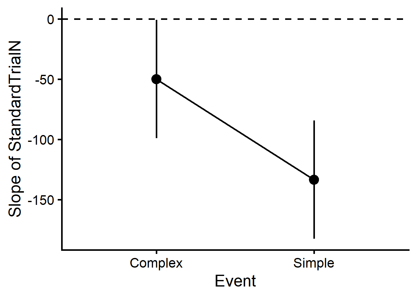
To visualize exactly how these slopes differ (and answer our LAST QUESTION!), we can include Event with the by= argument:
Slopes=estimate_slopes(mod, trend ='StandardTrialN', by ='Event')Slopes
Estimated Marginal Effects

Event   |   Slope |    SE |            95% CI | t(364) |      p
---------------------------------------------------------------
Complex |  -49.79 | 25.03 | [ -99.02,  -0.57] |  -1.99 |  0.047
Simple  | -133.39 | 25.01 | [-182.57, -84.21] |  -5.33 | < .001

Marginal effects estimated for StandardTrialN
Type of slope was dY/dX
Now we get the average effect for both Events. So we see that both of the lines significantly decrease!
Here we see that the slopes for both Conditions are negative (below zero) and that’s statistically significant (confidence intervals don’t cross the dashed zero line). This confirms that looking time reliably decreases as trials progress, regardless of whether it’s a Complex or Simple event.
Wrapping Up
Well, you did it! You’ve survived the wild jungle of model-based estimation! By breaking down the prediction process into customizable steps, you’ve gained complete control over how to extract and visualize the patterns in your eye-tracking data.
If you’re feeling like this is too much… well, it is. It was overwhelming even to just write the tutorial. Be gentle with your progress and don’t expect to know everything right away. Go through some of the steps again if need be. And reach out to us if somethings doesn’t make sense!
And most importantly: We hope it’s clear that any question you have about your data can be answered! It’s tricky or confusing at times, but you can follow this simple process:
think precsely at what your question is
think about what model would answer it
think about what contrasts will test your question directly
Don’t run models if your question is unclear, and don’t run contrasts on models you are not sure about.
Now you have the tools to answer sophisticated research questions and present your findings beautifully. Happy modeling!
---title: "Model Estimates"author: "Tommaso Ghilardi"date: "23/03/2025"description-meta: "Learn how to extract multiple information from your models. From estimate means, contrast and slopes!"keywords-meta: "R, lm, Linear models, statistics, analysis, psychology, tutorial, experiment, DevStart, developmental science"categories: - Stats - R - linear models---```{r}#| include: falseoptions(width =150)```Welcome back, stats adventurer! 👋 If you are here, it means you have already gone through our tutorial on: [Linear models](LinearModels.qmd), [Linear mixed effect models](LinearMixedModels.qmd). Well done!! You are nearly there, my young stats padawan. {style="margin-right:10px;margin-bottom:10px;" width="144"}You might think that once you’ve fit the model, you’re basically done: check the summary, look for stars, write the results. But there’s a catch: If we just look at `summary()`, we will know whether effects exist *(yes or no)*, but we still won't be able to *describe* them in detail.For example, if we find a significant interaction, we still don’t know the pattern that produced it. This is exactly what happened in our previous tutorial on mixed-effect models. Our hypothesis was simple: **looking time differs across conditions** (Simple vs Complex) but this difference **might change over trials**.::: {.callout-note title="Need a refresher?"}In our example paradigm, we designed a task where infants were presented with either a Simple or a Complex shape, and each shape was presented multiple times (that is, in multiple trials). We wanted to see if infants would look longer at the Complex shape, which would indicate increase interest for it over the Simple one. However, we were also mindful that this relationship might change (either get stronger or weaker) across trials. You can find an in-depth description of the experimental paradigm in our [intro tutorial](../EyeTracking/Intro_eyetracking.qmd).:::Even if we find a significant interaction between Condition (Simple vs Complex) and Trial Number, we still don't know what exactly is happening: is looking time significantly decreasing over trials in the Simple condition? Or is it increasing in the Complex condition? Or is looking time changing in both condition, but at different rates? Let's formulate our questions a bit more clearly:- *What is the difference in Looking Time between Simple and Complex condition?* ❓- *At which trials are the conditions reliably different?* ❓- *Are the slopes across trials significantly different between conditions?* ❓- *Is the change in looking time over trials significant for both conditions?* ❓Luckily for us, there is a solution to this: we can further *describe* what the main and interaction effects look like, and we can even confidently say - backed by statistics - which differences are significant.That's the goal of this next tutorial. We will show how to **visualise and test** the specific effects you care about using model-based **estimated means, contrasts, and slopes**, so you can make clear statements about *where* and *how* conditions differ!## Setting things up:::: {.columns}::: {.column width="55%"}First let's set things up to re-run our model. We import relevant libraries, read the data, set categorical variables as factors, standardize the continuous variables, and finally run our model.**Wait a sec, we just got an email...**I guess we have to listen to Reviewer #2 this time. Let's include an additional interaction with SES (Socio-Economic Status) in our model. This variable is a factor with 3 levels: high, medium, and low. The serendipitous thing is that this complex model will be useful to fully understand how model's predictions and estimates work, even when things get more complicated.:::::: {.column width="5%"}:::::: {.column width="40%"}::: {.callout-note title="Inbox"}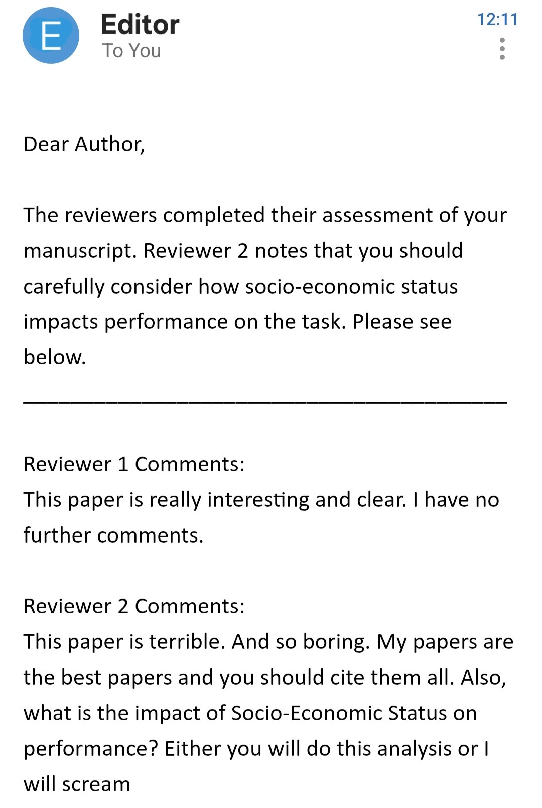::::::::::Here's our new model:```{r}#| label: Run model#| echo: true#| message: false#| warning: falselibrary(lme4)library(lmerTest)library(easystats)library(tidyverse)df =read.csv("resources/Stats/Dataset.csv")df$Id =factor(df$Id) # make sure subject_id is a factordf$SES =factor(df$SES) # make sure subject_id is a factordf$Event =factor(df$Event) # make sure subject_id is a factordf$StandardTrialN =standardize(df$TrialN) # create standardize trial columnmod =lmer(LookingTime ~ StandardTrialN * Event * SES + (1+ StandardTrialN | Id ), data= df)parameters(mod)```::: callout-cautionWe now have three variables interacting with each other (a three-way interaction). Be careful when adding too many interactions! As explained in this [blog post](https://datacolada.org/17), the sample size you need increases very quickly when you do that.Luckily for us, we are working on simulated data and, at least for these tutorials, we can get as much data as we want (\* evil laugh \*):::## Model predictionsRemember how easy it was to draw lines in the first tutorial on linear models!? Back then, a model with one or two predictors was something you could sketch by hand. But now, with **multiple interactions** and **random effects**, trying to “draw the model” with would quickly become a mess.Luckily, instead of pen and paper, we can ask the model to make **predictions** for us. That way, the model draws the lines while we sit back and relax. 😌Predictions are simply the values of `LookingTime` that the model expects under specific conditions (e.g., Simple vs Complex Condition, early vs late trials).We’ll use `estimate_expectation()` (from **modelbased**) to get predicted values directly from the fitted model. If we want to ask for predictions across Conditions and Trials, we can specify the following in the argument `by` (`length` tells how many values of the continuous predictor(s) to use):```{r}#| label: predictions-basic#| message: false #| warning: false library(modelbased)pred =estimate_expectation(mod, by =c("StandardTrialN", "Event"), length =15)head(pred)```As you can see, we get a Predicted value of looking time for each trial and event value! All without doing any mental arithmetics. Now we can plot these predictions to visualise the model-implied lines:```{r}#| label: predictions-plot #| message: false #| warning: false #| fig-height: 5.5#| fig-width: 8 plot(pred) +theme_classic(base_size =18) +theme(legend.position ="bottom")```Have you spotted anything odd in the previous output!??Well, look at the table with the model's predictions. Just below it, we see the following:`Predictors controlled: SES (high)`We gotta be careful! These predictions do not apply for all SES levels! When we ask for predictions “by Event and Trial”, the model still needs to decide what to do with *everything else* in the model (like `SES`, and the random effects). By default, predictions are computed at specific values (e.g., reference levels for factors), so they may not represent the “mean” effect you want to report.::: callout-tipIn this tutorial, we only introduce Prediction briefly because we care about means effects and contrasts more. However, you can always learn more on the [modelbased website](https://easystats.github.io/modelbased/articles/estimate_slopes.html) !!:::Predictions help us **describe** patterns (“the lines diverge”, “one looks steeper”), but they don’t directly answer the questions about our initial hypothesis we care about:- What is the average difference between Simple and Complex (overall, not at one SES level)? ❓- At which trials are the conditions reliably different? ❓- Are the slopes across trials significantly different between conditions? ❓- Is the change in looking time over trials significant for both conditions? ❓For that, we need model-based **estimates that are designed for inference**: **estimated means, contrasts, and slopes** - with uncertainty (CIs) and tests.In the next section, we’ll start with **estimated marginal means** (averaged over the other predictors), and then use **contrasts** to formally test the specific differences we care about.# Estimate meansAs its name suggests, `estimate_means()` allows you to extract estimated means from your model. But what does this actually mean? (Yes, lots of "means" in this explanation!)This function:1. Generates predictions for all the reference levels of a model's predictors2. Averages these predictions to keep only the predictors we are interested inThink of it as a streamlined way to answer the question: "What is the average looking time for each level of my factor, according to my model?" Let's see it in action!!```{r}#| label: EstMeansFactor#| message: false#| warning: falseEst_means =estimate_means(mod, by='Event')print(Est_means)```Notice the information message! Previously, with `estimate_expectation()`, we were setting SES to its reference level ("high"). **Now instead, the function extracts predictions for all levels of SES and then averages across them!**, giving you a comprehensive view of how Event influences looking behavior.\THIS IS WHAT WE WANTED!!! 🎉🎉🎉::: callout-note`estimate_expectation()` and `estimate_means()` handle the random effect structure differently. By default, `estimate_means()` gives us an average effect of the predictor for an average subject - exactly what we need when trying to understand overall patterns in our data. Learn more with [this vignette](https://easystats.github.io/modelbased/articles/mixed_models.html):::### Easy plottingThe `estimate_means()` function also comes with its own built-in plotting capability, automatically generating a clean ggplot visualization of your estimated means.```{r}#| label: PlotEstMean#| message: false#| warning: false#| fig-height: 5.5#| fig-width: 8plot(Est_means)+theme_classic(base_size =20)+theme(legend.position ='bottom')```# Estimate contrastsWe've successfully extracted and plotted the estimated means for our predictors - awesome job! 🎉**But there's something important missing**. While we now know the estimated looking times for each level, we don't yet have formal statistical comparisons between these levels. For example, is the difference between mean values in Complex condition and Simple condition statistically significant?This is where `estimate_contrasts()` comes to the rescue! Let's see it in action:```{r}#| label: ContrastCategorical#| warning: falseContrast =estimate_contrasts(mod, contrast ='Event')print(Contrast)```What we're doing here is simple but powerful:1. We pass our model to the function2. We specify which predictor we want to compare (Event)3. The function returns the difference between the means of the predictors with statistical testsThe results show us that the difference between Complex and Simple is positive (meaning looking time is higher for Complex) and the p-value indicates this difference is statistically significant! All of this with just one line of code - how convenient!In this example, Event has only 2 levels (Complex and Simple), so we already knew these levels differed significantly from examining our model summary. However, `estimate_contrast()` becomes particularly powerful when dealing with predictors that have multiple levels. With a predictor like **SES** (3 levels) - `estimate_contrast()` automatically calculates all possible pairwise comparisons between these levels.::: callout-noteRemember that if you have multiple levels in predictors you will need to adjust the *p-value* for multiple comparisons. You can do that by passing the argument `p_adjust = 'hochberg'` to the function. There are different adjustment methods and you can [check them here](https://easystats.github.io/modelbased/reference/estimate_contrasts.html).:::Let's run it on SES!!```{r}#| message: false#| warning: falseestimate_contrasts(mod, contrast ='SES',p_adjust ='hochberg')```See?? We have all the comparison between the available level of SES. Ough, nothing is significant here - Reviewer #2 really made us work for nothing. Well, hopefully it'll make them happy to know we listended to them. **And on the upside, if we will even need to test differences between 3 or more groups, we'll know exactly how to do that!**### Almost-as-Easy plotting`estimate_contrast()` has a plotting function as well! However, it's slightly more complex as the plot function requires both our estimated **contrasts** and **means**. If we pass both, the plot will show which level is different from the other using lighthouse plots - visualizations that highlight significant differences between groups.```{r}#| label: PlotContrasts#| message: false#| warning: false#| fig-height: 5.5#| fig-width: 8plot(Contrast, Est_means)+theme_classic(base_size =20)+theme(legend.position ='bottom')```## InteractionsWe hope you are getting a hang of how `estimate_contrast()` works. It helped us testing the first part of our hypothesis (and even check the effect of SES), but if we look back at our questions, two more aspects are still unclear:- What is the average difference between Simple and Complex (overall, not at one SES level)? ✅**About 300ms, and the difference is significant!**- At which trials are the conditions reliably different? ❓- Are the slopes across trials significantly different between conditions? ❓- Is the change in looking time over trials significant for both conditions? ❓Luckily for us, `estimate_contrast()` really shines the most when examining interactions between categorical and continuous predictors - just what we want. More specifically, we care about whether the effect of Condition (`Event`), changes across Trials. So we can keep `contrast = Event`. But now we also want to compute that difference across trials! For that, we can use `by =`. Here's how it works:- `contrast =` tells the function **what difference you want to compute** (e.g., Complex vs Simple).- `by =` tells it **where to compute that difference** (at different trial values).```{r}#| label: SlopeFactorContinuos#| warning: false#| fig-height: 10#| fig-width: 10#| paged-print: falseContrastbyTrial =estimate_contrasts(mod, contrast ='Event', by ='StandardTrialN', p_adjust ='hochberg')ContrastbyTrial```This gives us the contrast between the levels of `Event` for a set of values of StandardTrialN. So we can check whether the difference between Complex and Simple actually changes over the course of trials!! We'll plot it to make it simpler to understand:```{r}#| label: PlotContrastInteraction#| echo: false#| message: false#| warning: false#| fig-height: 6#| fig-width: 8.5ContrastbyTrial |>mutate(Contrast =paste(Level1, "-", Level2)) |>ggplot(aes(x = StandardTrialN , y = Difference, color = Contrast))+geom_hline(yintercept =0, linetype ='dashed')+geom_pointrange(aes(ymin = CI_low, ymax = CI_high))+labs(y ='Difference: Complex - Simple')+theme_classic(base_size =20)+theme(legend.position ='bottom')```This plot shows that the two levels are always significantly different from each other (the confidence intervals never touch the dashed zero line) and that the difference is always positive - looking time for Complex is consistently higher than for Simple across all trial numbers. SUUPER COOL, EH!!?::: callout-importantYou *can* put multiple predictors in `contrast =` (it will compute lots of pairwise differences across combinations), but be careful: the number of tests can explode fast... and you’ll want p-value adjustment.:::# Comparing slopesWow, it took a while to get here, but now we're quickly answering all of our questions! We're already half-way through:- What is the average difference between Simple and Complex (overall, not at one SES level)? ✅**About 300ms, and the difference is significant!**- At which trials are the conditions reliably different? ✅**All of them!**- Are the slopes across trials significantly different between conditions? ❓- Is the change in looking time over trials significant for both conditions? ❓To answer the next question, we can again use the `estimate_contrast()` function. However, we need to make a fundamental change. Before, we cared about how the effect of Condition changed across Trials. Now, we care about how the effect of Trial changes across conditions!Is that super confusing? It still is for us, sometimes. But remembering our question helps: Does the effect of time (Trial) change across Conditions? For that, our main interest is Trial Number, and we want to see how the experimental condition modulates it. So StandardTrialN moves to the contrast argument and Event goes to the by argument:```{r}#| label: ContrastFactorContinuos#| message: false#| warning: falseestimate_contrasts(mod, contrast ='StandardTrialN', by ='Event')```This shows us that the effect of StandardTrialN is actually different between the two levels. This is something we already knew from the model summary (remember the significant interaction term?), but this approach gives us the precise difference between the two slopes while averaging over all other possible effects. This becomes particularly valuable when working with more complex models that have multiple predictors and interactions.# Estimate SlopesYay, only one question left!!- What is the average difference between Simple and Complex (overall, not at one SES level)? ✅**About 300ms, and the difference is significant!**- At which trials are the conditions reliably different? ✅**All of them!**- Are the slopes across trials significantly different between conditions? ✅**Yes! (we new this already, actually)**- Is the change in looking time over trials significant for both conditions? ❓To answer this one, there's one last very important function worth introducing: `estimate_slope()`. While `estimate_means()` allows us to extract the means of predictions, `estimate_slope()` is designed specifically for understanding rates of change.This will help us understand *how quickly* looking time changes across trials in the two conditions. Here, the key argument is `trend =`. In our case, we are interested in changes across time, so we put trial number here:```{r}#| label: EstSlope#| warning: falseestimate_slopes(mod, trend ='StandardTrialN')```This tells us that the average effect of StandardTrialN is -50.46 (negative) and it is significantly different from 0. This means the looking time doesn't remain constant across trials but significantly decreases as trials progress.::: callout-importantYou may be thinking... "Wait, isn't this information already in the model summary? Why do I need `estimate_slopes()`?" If you are asking yourself this question, think back to the [Linear models](LinearModels.qmd) tutorial!!**What the model summary shows:** The coefficient for StandardTrialN in the summary (-67.118) represents the slope specifically for the Simple condition. This is because in linear models, coefficients are in relation to the intercept, which is where all predictors are 0. For categorical variables, 0 means the reference level (Simple in this case).**What estimate_slopes() shows:** The value from `estimate_slopes()` (-50.46) gives us the average slope across both Event types (Complex and Simple).This is why the two values don't match! One is the slope for a specific condition, while the other is the average slope across all conditions. Super COOL right??:::Remember! Our model indicated an interaction between StandardTrialN and Event, which means the rate of change (slope) should differ between the two Event types. However, from just knowing there's an interaction, we can't determine exactly what these slopes are doing. One condition might show a steeper decline than the other, one might be flat while the other decreases, or they might even go in opposite directions. The model just tells us they're different, not how they're different (or at least it is not so simple)To visualize exactly how these slopes differ (and answer our LAST QUESTION!), we can include `Event` with the `by=` argument:```{r}Slopes =estimate_slopes(mod, trend ='StandardTrialN', by ='Event')Slopes```Now we get the average effect for both Events. So we see that both of the lines significantly decrease!We can also plot it with:```{r}plot(Slopes)+geom_hline(yintercept =0, linetype ='dashed')+theme_classic(base_size =20)+theme(legend.position ='bottom')```Here we see that the slopes for both Conditions are negative (below zero) and that's statistically significant (confidence intervals don't cross the dashed zero line). This confirms that looking time reliably decreases as trials progress, regardless of whether it's a Complex or Simple event.# Wrapping UpWell, you did it! You've survived the wild jungle of model-based estimation! By breaking down the prediction process into customizable steps, you've gained complete control over how to extract and visualize the patterns in your eye-tracking data.If you're feeling like this is too much... well, it is. It was overwhelming even to just write the tutorial. Be gentle with your progress and don't expect to know everything right away. Go through some of the steps again if need be. And reach out to us if somethings doesn't make sense!And most importantly: We hope it's clear that any question you have about your data can be answered! It's tricky or confusing at times, but you can follow this simple process:- think precsely at what your *question* is- think about what *model* would answer it- think about what *contrasts* will test your question directlyDon't run models if your question is unclear, and don't run contrasts on models you are not sure about.Now you have the tools to answer sophisticated research questions and present your findings beautifully. Happy modeling!