import os
from pathlib import Path
import numpy as np
import pandas as pd
import matplotlib.pyplot as plt
import matplotlib.patches as patches

#%% Settings

# Screen resolution
screensize = (1920, 1080)

#%% Settings and reading data

# Define paths using pathlib
base_path = Path('resources/FromFixationToData/DATA')

# The fixation data extracted from I2MC
Fixations = pd.read_csv(base_path / 'i2mc_output' / 'Adult1' / 'Adult1.csv')

# The original RAW data
Raw_data = pd.read_hdf(base_path / 'RAW' / 'Adult1.h5', key='gaze')From fixations to measures
Eye-tracking
Python
Keywords
Python, latency, saccadic-latency, looking time, eye-tracking, tobii, experimental psychology, tutorial, experiment, DevStart, developmental science
In the previous two tutorials we collected some eye-tracking data and then we used I2MC to extract the fixations from that data. Let’s load the data we recorded and pre-processed in the previous tutorial. We will import some libraries and read the raw data and the output from I2MC.
What can we do with just the raw data and the fixations? Not much I am afraid. But we can use these fixations to extract some more meaningful indexes.
In this tutorial, we will look at how to extract two variables from our paradigm:
Saccadic latency: how quickly our participant looked at the correct location. This includes checking whether the participant could anticipate the stimulus appearance. In our paradigm, we will look at how fast our participant looked at the target location (left: Simple stimulus, right: Complex stimulus).
Looking time: how long our participant looked at certain locations on the screen. In our case, we will look at how long our participant looked at either target location (left: Simple stimulus, right: Complex stimulus) on each trial.
So what do these two measures have in common? pregnant pause for you to answer EXACTLY!!! They are both clearly related to the position of our stimuli. For this reason, it is important to define Areas Of Interest (AOIs) on the screen (for example, the locations of the targets). Defining AOIs will allow us to check, for each single fixation, whether it happened in an area that we are interested in.
Areas Of Interest
Define AOIs
Let’s define AOIs. We will define two squares around the target locations. To do this, we can simply pass two coordinates for each AOI: the lower left corner and the upper right corner of an imaginary square.
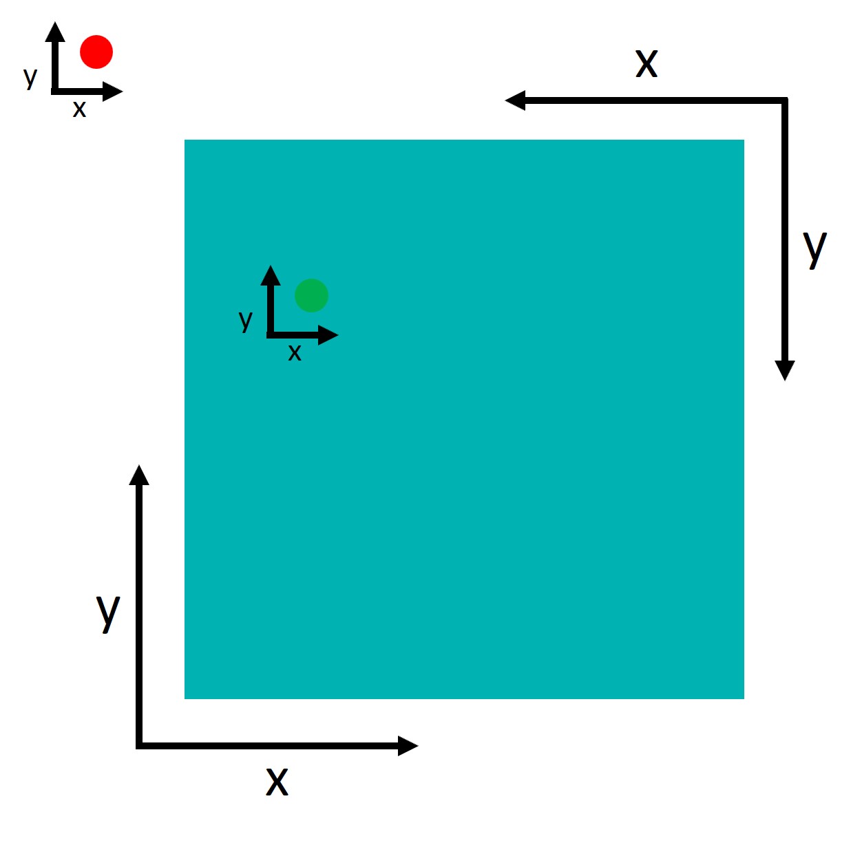
An important point to understand is that tobii and Psychopy use two different coordinate systems:
Psychopy has its origin (0,0) in the centre of the window/screen by default.
Tobii reports data with its origin (0,0) in the lower left corner.
This inconsistency is not a problem per se, but we need to take it into account when defining the AOIs. Let’s try to define the AOIs:
# Screen resolution
screensize = (1920, 1080)

# Define variables related to AOIs and target position
dimension_of_AOI = 600/2  # half-width of the square
Target_position = 500     # distance from center (pixels)

# Create Areas of Interest (AOIs)
# Format: [[bottom_left_x, bottom_left_y], [top_right_x, top_right_y]]

# AOI 1: Left Target (Negative X)
# Center is (-500, 0)
AOI1 = [
    [-Target_position - dimension_of_AOI, -dimension_of_AOI], # Bottom-Left
    [-Target_position + dimension_of_AOI,  dimension_of_AOI]  # Top-Right
]

# AOI 2: Right Target (Positive X)
# Center is (+500, 0)
AOI2 = [
    [Target_position - dimension_of_AOI, -dimension_of_AOI],  # Bottom-Left
    [Target_position + dimension_of_AOI,  dimension_of_AOI]   # Top-Right
]

AOIs = [AOI1, AOI2]
Nice!! This step is essential. We have created two AOIs. We will use them to define whether each fixation of our participant was within either of these two AOIs. Let’s get a better idea by just plotting these two AOIs and two random points (600, 500) and (1400,1000).
Code
import matplotlib.pyplot as plt
import matplotlib.patches as patches

# Create a figure
fig, ax = plt.subplots(1, figsize=(8, 4.4))

# Set the limits of the plot (Center origin!)
# X: -960 to 960
# Y: -540 to 540
ax.set_xlim(-screensize[0]/2, screensize[0]/2)
ax.set_ylim(-screensize[1]/2, screensize[1]/2)

# Define the colors for the rectangles
colors = ['#46AEB9', '#C7D629']

# Add axes lines to show the center (0,0) clearly
ax.axhline(0, color='gray', linestyle='--', alpha=0.5)
ax.axvline(0, color='gray', linestyle='--', alpha=0.5)

# Create a rectangle for each area of interest and add it to the plot
for i, (bottom_left, top_right) in enumerate(AOIs):
    width = top_right[0] - bottom_left[0]
    height = top_right[1] - bottom_left[1]

    rectangle = patches.Rectangle(
        bottom_left, width, height,
        linewidth=2, edgecolor='k', facecolor=colors[i], alpha=0.6
    )
    ax.add_patch(rectangle)

# Plot random points to test (e.g., one inside Left AOI, one inside Right AOI)
# Note: These coordinates are now relative to center!
# (-600, 0) is inside the Left AOI
# (600, 0) is inside the Right AOI
ax.plot(-500, 0, marker='o', markersize=8, color='white', label='Left Target Center')
ax.plot(500, 0, marker='o', markersize=8, color='white', label='Right Target Center')

# Show the plot
plt.title("AOIs")
plt.show()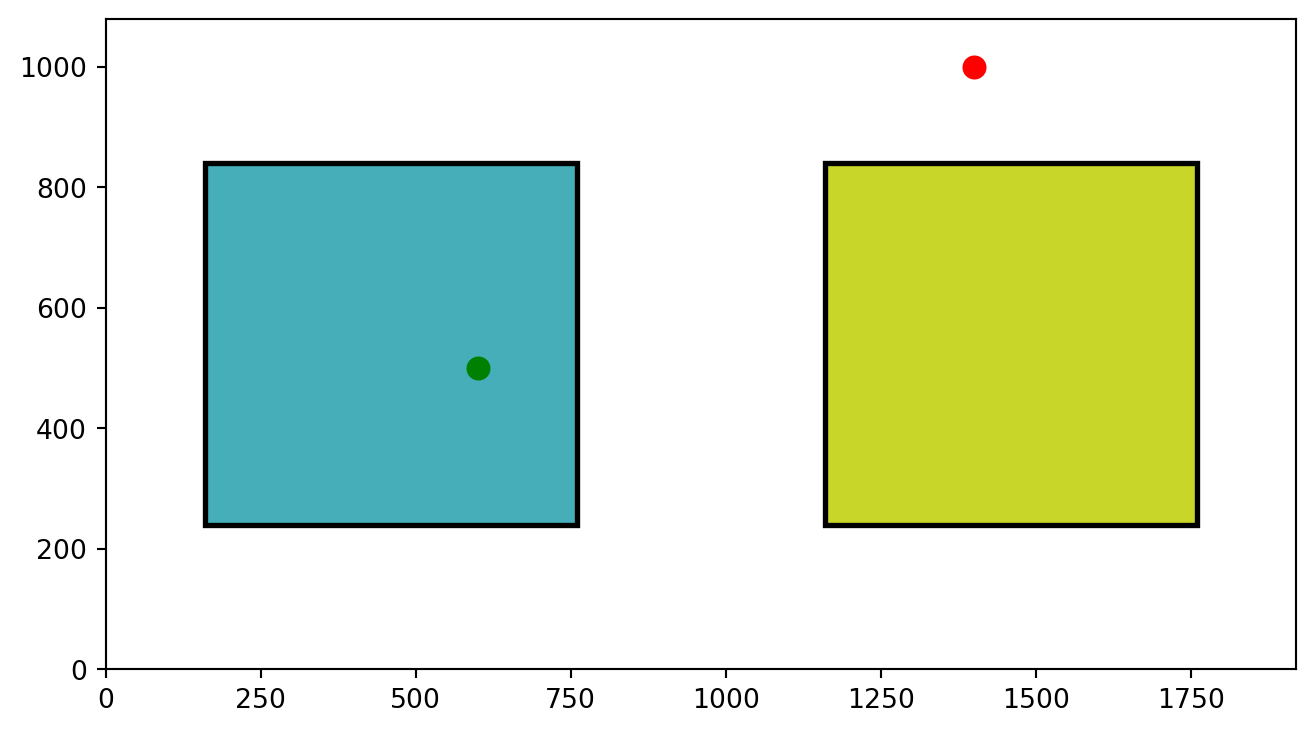
Points in AOIs
As you can see from our plot, we have two defined Areas of Interest (AOIs). Visually, it is obvious which points would fall inside the boxes and which do not. But how do we get Python to determine this mathematically?
The logic is actually quite simple. We just need to check if the point’s coordinates lie within the boundaries of the rectangle:
Is the point’s X between the rectangle’s Left and Right edges?
Is the point’s Y between the rectangle’s Bottom and Top edges?
Here is the basic logic for checking a single area:
So imagine we have a point: point and an area: area, we can check if the point falls inside the area by:
# 1. Extract the rectangle boundaries
bottom_left, top_right = area
min_x, min_y = bottom_left
max_x, max_y = top_right

# 2. Extract the gaze point coordinates
x, y = point

# 3. Check if the point is inside boundaries
is_inside = (min_x <= x <= max_x) and (min_y <= y <= max_y)
Perfect, this will return True if the point falls inside the area and False if it falls outside.
Checking Multiple AOIs
Since we have two targets (Left and Right), simply knowing “True/False” isn’t enough. We need to know which specific AOI the participant was looking at.
To do this, we will build a function called find_area_for_point. Instead of returning a boolean, this function will return an index:
0if the point is in the first AOI (Left Target).1if the point is in the second AOI (Right Target).-1if the point is essentially “nowhere” (looking at the background).
We achieve this using Python’s enumerate function.
More details
Normally, looping through a list (for area in areas) gives you the items one by one but forgets their position. enumerate solves this by giving us two things simultaneously:
The Index (i): The ID number of the item (0, 1, 2…).
The Item (area): The actual coordinates of the AOI.
This is perfect for us: we use the Item to do the math (checking if the point is inside), and if it is, we return the Index so we know which target was looked at.
# We define a function that simply takes the a point and a list of areas.
# This function checks in which area this point is and return the index
# of the area. If the point is in no area it returns -1
def find_area_for_point(point, areas):
    """
    Checks which AOI a point falls into.
    Returns the index of the AOI, or -1 if the point is outside all areas.
    """
    for i, area in enumerate(areas):
        # Extract boundaries
        bottom_left, top_right = area
        min_x, min_y = bottom_left
        max_x, max_y = top_right

        # Extract point
        x, y = point

        # Check boundaries
        if (min_x <= x <= max_x) and (min_y <= y <= max_y):
            return i

    # If the loop finishes without returning, the point is outside all AOIs
    return -1
Now we have a cool function to check whether a point falls into any of our AOIs. We can use this function to filter the fixations that are in the AOIs: These are the only ones we care about.
Time Of Interest
Now that we’ve figured out how to select fixations that fall within our areas of interest, it’s time to consider another important factor: Time. Our experiment involves presenting a variety of stimuli, including fixation crosses, cues, and target stimuli. , we’re not interested in analyzing the entire experiment. Instead, we focus on specific events.
Let’s take a look at the design image. What we are interest in is the last part, the target presentation.
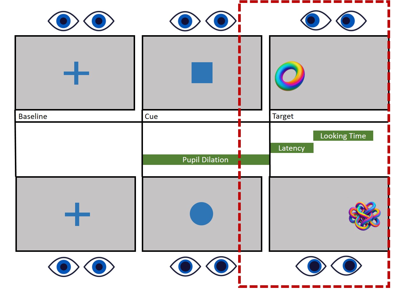
In this case, our attention is on the target window. We’re going to establish a time window that begins 750ms before the target appears and continues for 2000ms after its presentation. Indeed, both Saccadic latency and Lookign time occur within this time window, while we don’t really care about where the participant is looking during other phases of the task.
Let’s start by finding the moment in which the target appeared:
# Define the events we are interested in
target_labels = ['Complex', 'Simple']

# Filter the Raw Data to find rows where these events occurred
# We select the 'TimeStamp' (when it happened) and the 'Events' (label)
Targets = Raw_data.loc[
    Raw_data['Events'].isin(target_labels),
    ['TimeStamp', 'Events']
].values
Having identified exactly when the targets appeared (the Targets list we just created), we need to link this information to our fixations.
Currently, our Fixations dataframe just has a list of start times (startT). It doesn’t know that the fixation starting at 4500ms belongs to “Trial 1” or that the participant was looking at a “Complex” stimulus.
To fix this, we will iterate through our list of targets one by one. For each target, we create a temporary “time window” around its onset (from -750ms to +2000ms). Then, we check if any fixations started inside that window.
If a fixation falls inside the window, we “tag” it with three pieces of information:
Events: The label of the stimulus (e.g., ‘Complex’). We use “Events” (plural) to match the DeToX column name.
TrialN: The trial number (0, 1, 2…). This is crucial for separating the same condition across different times.
Onset: The exact timestamp when the target appeared. We need this later to calculate Reaction Times (Fixation Start Time - Target Onset Time).
Here is the code to do exactly that:
# Find the fixations that we care about
pre  = -750
post = 2000

# Loop through each target
# trial_idx   = The specific trial number (0, 1, 2...)
# target_data = The row containing [Time, Label] for this target
for trial_idx, target_data in enumerate(Targets):

    # 1. Create a "mask" to find fixations in the specific time window
    mask = (Fixations['startT'] >= target_data[0] + pre) & (Fixations['startT'] < target_data[0] + post)

    # 2. Tag these fixations with the trial info

    Fixations.loc[mask, 'Events'] = target_data[1] # Save the Event (e.g., 'Complex')
    Fixations.loc[mask, 'TrialN'] = trial_idx # Save the Trial Number
    Fixations.loc[mask, 'Onset'] = target_data[0] # Save the Onset Time
Our Fixations dataframe is now populated with event details, but it still contains data we don’t need. Specifically, any fixation that occurred outside our defined time windows (e.g., during the break between trials) has NaN (empty values) in the new columns.
We can use this to our advantage! By filtering out these NaN values, we instantly remove all the irrelevant noise and create a clean dataset containing only the fixations that happened during the trials.
# We can drop the NANs to have only the fixations that interest us!!!!
Target_fixations = Fixations[Fixations['Events'].notna()].reset_index(drop=True)
Put things together
Now we have selected our fixations based on Time (the events). But we also need to filter them based on Space (the AOIs).
Luckily, we just built the find_area_for_point function to do exactly that!
As a first step, we will add a new column to our Target_fixations dataframe containing the AOIs we defined together before. Thus, each row of this column will tell us which AOIs we should check. We will also add a new column called Looked_AOI where we will store the indexes of which AOI the fixation fell into.
Important
Just a heads up: our study design is pretty straightforward with only two stable Areas of Interest (AOIs). But if you’re dealing with multiple or moving AOIs, you’ve got options. You can add them to each row of the dataframe, depending on the event or trial. This way, you get more control over which area to inspect at any given moment of the study. It’s all about flexibility and precision!
# 1. Add the AOI definitions to every row
# (Since our targets don't move, we add the same list to everyone)
Target_fixations['AOIs'] = [AOIs] * len(Target_fixations)

# 2. Create an empty column to store the result
Target_fixations['Looked_AOI'] = np.nan
Now we iterate through every fixation. For each row, we grab the gaze coordinates (xpos, ypos) and the AOIs, then ask our function: “Did this fixation land inside?”
# We run the function  for each row. We pass each xpos and ypos to the function
# toghether with the areas
for row in range(len(Target_fixations)):

    # Extract the gaze point (x, y)
    Point = Target_fixations.loc[row, ['xpos', 'ypos']].values

    # Extract the AOIs relevant for this trial
    Areas = Target_fixations.loc[row, 'AOIs']

    # Run our function and save the result (0, 1, or -1)
    Target_fixations.loc[row, 'Looked_AOI'] = find_area_for_point(Point, Areas)
Perfect, we now have a dataframe that contains only the fixations of interest and tells us which AOI each fixation is in.
The final step is to remove the “noise”—any fixation that returned -1. These are moments where the participant was looking at the screen, but not at either of our targets (e.g., looking at the background).
# Filter out fixations that missed the targets (where result is -1)
Target_fixations = Target_fixations[Target_fixations['Looked_AOI'] != -1]
Saccadic latency
As mentioned at the start of this tutorial, one of the key metrics we want to extract is Saccadic Latency. Essentially, this tells us how quickly our participants fixated on the correct target location after it appeared.
If we know where our participant was supposed to look, we can easily find their first correct fixation.
<<<<<<< HEAD In our specific paradigm, the stimuli were always presented in fixed locations:
Simple Stimulus: Always on the Left (AOI Index
0).Complex Stimulus: Always on the Right (AOI Index
1).
We can add this “ground truth” to our dataframe. Then, we simply compare it to where they actually looked (Looked_AOI). If the two match, it’s a correct fixation!
In our paradigm, the Simple stimulus was always presented on the left (the first AOI we defined) and the Complex stimulus was always presented on the right (the second AOI we defined). Thus we can add this information to our dataframe and then use it to filter out the wrong fixations: >>>>>>> TommasoGhilardi/issue26
# 1. Define the Correct AOI for each condition
# Simple -> Left (AOI 0)
Target_fixations.loc[Target_fixations['Events'] == 'Simple', 'Correct_Aoi'] = 0

# Complex -> Right (AOI 1)
Target_fixations.loc[Target_fixations['Events'] == 'Complex', 'Correct_Aoi'] = 1

# 2. Filter: Keep only the fixations where they looked at the Correct AOI
Correct_Target_fixations = Target_fixations.loc[
    Target_fixations['Correct_Aoi'] == Target_fixations['Looked_AOI']
].copy() # We use .copy() to avoid SettingWithCopy warnings later
Now comes the easy part. To find the latency (reaction time), we simply subtract the time the Target appeared (Onset) from the time the Fixation started (startT).
# Calculate Latency: Fixation Start Time - Target Appearance Time
Correct_Target_fixations['Latency'] = Correct_Target_fixations['startT'] - Correct_Target_fixations['Onset']
Et voilà! It’s that simple. Your Latency column now contains the reaction time in milliseconds for every correct fixation.
Note
Can Latency be negative? Yes! A negative latency means the participant looked at the target location before the target actually appeared. This indicates that they successfully predicted the location and moved their eyes in anticipation. In many studies, measuring this anticipation is exactly why we use saccadic latency!
First fixation
We now have a list of all correct fixations, but often there are multiple fixations within a single trial (e.g., the participant looks at the target, looks away, then looks back).
For Saccadic Latency, we care only about the first time they looked at the target. That is their reaction time.
How do we isolate just that one specific row for every trial? We use the powerful groupby function in pandas.
groupby allows us to split our dataframe into small chunks (one chunk per Trial), find the minimum value in each chunk (the smallest Latency = the earliest fixation), and glue it all back together.
# Group the data by 'Events' (Condition) and 'TrialN' (Trial Number)
# Then find the minimum (.min) Latency in each group
SaccadicLatency = Correct_Target_fixations.groupby(['Events', 'TrialN'])['Latency'].min().reset_index()
Mission Accomplished! You now have a clean dataframe containing exactly one latency value per trial.
Finally, let’s see what our data looks like! We can use the seaborn library to create a beautiful scatterplot showing how saccadic latency changes across the trials.
import seaborn as sns
import matplotlib.pyplot as plt

plt.figure(figsize=(8, 6))

# Create the scatterplot
# x = Trial Number
# y = Latency (Reaction Time)
# hue = Color points differently based on the Event (Simple vs Complex)
ax = sns.scatterplot(
    data=SaccadicLatency,
    x="TrialN",
    y="Latency",
    hue='Events',
    style='Events',   # Different shapes for different events
    s=100             # Make the dots bigger
)

# Move the legend to a clean spot
sns.move_legend(ax, "upper left", bbox_to_anchor=(1, 1))

plt.title("Saccadic Latency across Trials")
plt.ylabel("Latency (ms)")
plt.xlabel("Trial Number")
plt.tight_layout()

# Show the plot
plt.show()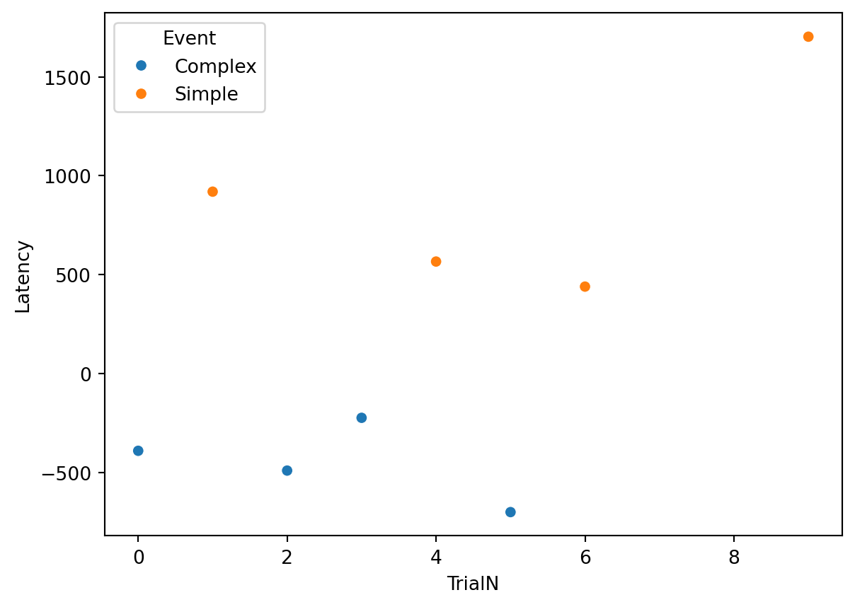
Looking time
While our paradigm was designed with saccadic latency in mind, we can also extract Looking Time. This measure tells us the total duration the participant spent looking at a specific Area of Interest (AOI) during each trial.
We have already extracted all the necessary raw data; we just need to aggregate it.
Again, we use groupby. We group our dataframe by Events (Condition), TrialN (Trial Number), and Looked_AOI (Location). Then, we sum the duration (dur) of all fixations in that group.
# Calculate Total Looking Time per AOI, per Trial, per Event
LookingTime = Target_fixations.groupby(
    ['Events', 'TrialN', 'Looked_AOI'],
    as_index=False
)['dur'].sum()
Now we can visualize the results. For instance, we can compare the average looking time directed at the Simple stimulus versus the Complex stimulus.
Since sns.barplot automatically calculates the mean and confidence intervals (error bars), it is perfect for seeing if there is a statistically significant difference in how long participants looked at the two types of images.
plt.figure(figsize=(6, 5))

# Create a bar plot
# y = Duration (How long they looked)
# x = Events (Simple vs Complex)
# We filter LookingTime to only include the "Correct" AOI for the intended stimulus
# (Remember: Simple is AOI 0, Complex is AOI 1)
# For this plot, we assume we want to know time spent on the TARGET itself.

ax = sns.barplot(
    data=LookingTime,
    y="dur",
    x="Events",
    hue="Events",
    palette=['#46AEB9', '#C7D629'] # Use custom colors for style
)

ax.set_ylabel("Total Looking Duration (ms)")
ax.set_xlabel("Stimulus Type")
ax.set_title("Looking Time: Simple vs Complex")

# Show the plot
plt.show()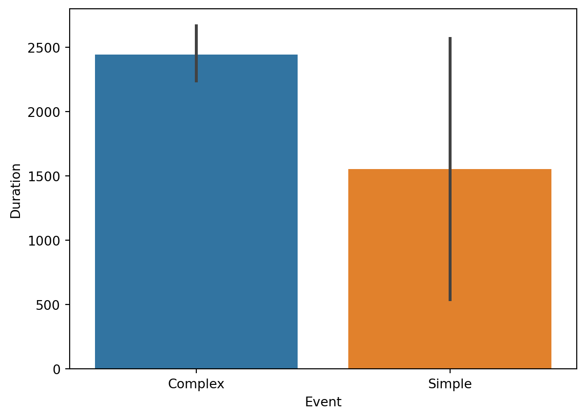
END!!
Well done!! we have successfully extracted both saccadic latency and looking time from our data. Remember that it is just a simple tutorial based on an even simpler design. However, if you got to the end and you have understood all the steps and what they mean, I am sure you can apply this knowledge to your study as well. If you have any questions or if something is not clear, feel free to send us an email!!
Here below the entire script!!
import os
from pathlib import Path
import numpy as np
import pandas as pd
import seaborn as sns
import matplotlib.pyplot as plt
import matplotlib.patches as patches

#%% Functions

def find_area_for_point(point, areas):
    """
    Checks which AOI a point falls into.
    Returns the index of the AOI (0, 1, etc.), or -1 if outside all areas.
    """
    for i, area in enumerate(areas):
        # Extract boundaries (bottom_left, top_right)
        bottom_left, top_right = area
        min_x, min_y = bottom_left
        max_x, max_y = top_right

        # Extract point coordinates
        x, y = point

        # Check if point is inside
        if (min_x <= x <= max_x) and (min_y <= y <= max_y):
            return i

    # If the loop finishes without returning, the point is outside all AOIs
    return -1


#%% Setup and Loading Data

# Screen resolution (width, height)
screensize = (1920, 1080)

# Define paths
base_path = Path('resources/FromFixationToData/DATA')

# 1. Load Fixations (Output from I2MC)
fixations_path = base_path / 'i2mc_output' / 'Adult1' / 'Adult1.csv'
Fixations = pd.read_csv(fixations_path)

# 2. Load Raw Data (Output from DeToX)
raw_data_path = base_path / 'RAW' / 'Adult1.h5'
Raw_data = pd.read_hdf(raw_data_path, key='gaze')


#%% Define Areas of Interest (AOIs)

dimension_of_AOI = 600/2   # Half-width of the square
Target_position = 500      # Distance from center in pixels

# AOI 1: Left Target (Simple Stimulus) -> Negative X
AOI1 = [
    [-Target_position - dimension_of_AOI, -dimension_of_AOI], # Bottom-Left
    [-Target_position + dimension_of_AOI,  dimension_of_AOI]  # Top-Right
]

# AOI 2: Right Target (Complex Stimulus) -> Positive X
AOI2 = [
    [Target_position - dimension_of_AOI, -dimension_of_AOI],  # Bottom-Left
    [Target_position + dimension_of_AOI,  dimension_of_AOI]   # Top-Right
]

AOIs = [AOI1, AOI2]

# Visualization Check
fig, ax = plt.subplots(1, figsize=(8, 4.4))
ax.set_xlim(-screensize[0]/2, screensize[0]/2)
ax.set_ylim(-screensize[1]/2, screensize[1]/2)
colors = ['#46AEB9', '#C7D629']

ax.axhline(0, color='gray', linestyle='--', alpha=0.5)
ax.axvline(0, color='gray', linestyle='--', alpha=0.5)

for i, (bottom_left, top_right) in enumerate(AOIs):
    width = top_right[0] - bottom_left[0]
    height = top_right[1] - bottom_left[1]
    rect = patches.Rectangle(bottom_left, width, height, linewidth=2, edgecolor='k', facecolor=colors[i], alpha=0.6)
    ax.add_patch(rect)

plt.title("AOIs Check (Center Origin)")
plt.show()


#%% Time of Interest (Matching Events)

# Define the labels we are looking for
target_labels = ['Complex', 'Simple']

# Extract rows where targets appeared
Targets = Raw_data.loc[
    Raw_data['Events'].isin(target_labels),
    ['TimeStamp', 'Events']
].values

# Define the analysis window around the target onset (ms)
pre  = -750
post = 2000

# Loop through each target
# trial_idx   = The specific trial number (0, 1, 2...)
# target_data = The row containing [Time, Label] for this target
for trial_idx, target_data in enumerate(Targets):

    # 1. Create a "mask" to find fixations in the specific time window
    mask = (Fixations['startT'] >= target_data[0] + pre) & (Fixations['startT'] < target_data[0] + post)

    # 2. Tag these fixations with the trial info

    Fixations.loc[mask, 'Events'] = target_data[1] # Save the Event (e.g., 'Complex')
    Fixations.loc[mask, 'TrialN'] = trial_idx # Save the Trial Number
    Fixations.loc[mask, 'Onset'] = target_data[0] # Save the Onset Time

# Filter: Drop fixations that didn't happen during a target trial
Target_fixations = Fixations[Fixations['Events'].notna()].reset_index(drop=True)


#%% Spatial Filtering (Checking points in AOIs)

# Add the AOI definitions to every row
Target_fixations['AOIs'] = [AOIs] * len(Target_fixations)
Target_fixations['Looked_AOI'] = np.nan

# Loop through every fixation to check its location
for row in range(len(Target_fixations)):

    # Get gaze coordinates
    Point = Target_fixations.loc[row, ['xpos', 'ypos']].values
    # Get areas for this trial
    Areas = Target_fixations.loc[row, 'AOIs']

    # Check location
    Target_fixations.loc[row, 'Looked_AOI'] = find_area_for_point(Point, Areas)

# Filter: Remove fixations that missed the targets
Target_fixations = Target_fixations[Target_fixations['Looked_AOI'] != -1]


#%% Saccadic Latency Analysis

# 1. Define Ground Truth
Target_fixations.loc[Target_fixations['Events'] == 'Simple', 'Correct_Aoi'] = 0
Target_fixations.loc[Target_fixations['Events'] == 'Complex', 'Correct_Aoi'] = 1

# 2. Select only Correct Fixations
Correct_Target_fixations = Target_fixations.loc[
    Target_fixations['Correct_Aoi'] == Target_fixations['Looked_AOI']
].copy()

# 3. Calculate Latency
Correct_Target_fixations['Latency'] = Correct_Target_fixations['startT'] - Correct_Target_fixations['Onset']

# 4. Extract First Fixation per Trial
SaccadicLatency = Correct_Target_fixations.groupby(['Events', 'TrialN'])['Latency'].min().reset_index()

# Plot Latency
plt.figure(figsize=(8, 6))
ax = sns.scatterplot(
    data=SaccadicLatency,
    x="TrialN", y="Latency", hue='Events', style='Events', s=100
)
sns.move_legend(ax, "upper left", bbox_to_anchor=(1, 1))
plt.title("Saccadic Latency across Trials")


#%% Looking Time Analysis

# Sum duration of all fixations per Trial and Event
LookingTime = Target_fixations.groupby(
    ['Events', 'TrialN', 'Looked_AOI'],
    as_index=False
)['dur'].sum()

# Plot Looking Time
plt.figure(figsize=(6, 5))
ax = sns.barplot(
    data=LookingTime,
    x="Events", y="dur", hue="Events",
    palette=['#46AEB9', '#C7D629']
)
ax.set_ylabel("Total Looking Duration (ms)")
plt.title("Looking Time: Simple vs Complex")
plt.show()